VLOOKUP Formula : How to do a VLOOKUP step by step

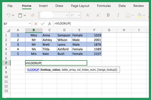
The VLOOKUP formula is a popular function in Microsoft Excel used to search for a specific value in a vertical column and retrieve information from a corresponding column. 

Let's break down the components of the formula:

lookup_value: 

This is the value you want to find in the leftmost column of the table or range.

table_array: 

This is the range of cells that contains the data you want to search in. It should include the column where the lookup value is located and the column from which you want to retrieve information.

col_index_num: 

This specifies the column number in the table_array from which you want to retrieve data. The leftmost column is numbered as 1, the next column as 2, and so on.

range_lookup: 

This is an optional parameter that specifies whether you want an exact match or an approximate match. If set to TRUE or omitted, an approximate match will be used (sorted column required); if set to FALSE, an exact match will be performed.

In this example, we're searching for the value in cell A2 within the range Sheet2!A2:B10. If a match is found, the corresponding value from the second column of the range will be retrieved. The FALSE argument indicates that we want an exact match.

Remember to adjust the cell references and table ranges as per your specific needs.

How to do a VLOOKUP step by step

Sure! Let's go through the steps of performing a VLOOKUP in Excel:

Step 1: Understand the data

Make sure you understand the structure of your data and know which value you want to look up and which column you want to retrieve data from.

Step 2: Set up your worksheet

Ensure that your data is organized in a table format with column headers and the relevant information you need to retrieve.

Step 3: Determine the lookup value

Identify the value you want to search for in the leftmost column of your table.

Step 4: Identify the table range

Determine the range of cells that contains your data. This range should include the lookup column and the column(s) from which you want to retrieve information.

Step 5: Write the VLOOKUP formula

In an empty cell, enter the VLOOKUP formula using the syntax: =VLOOKUP(lookup_value, table_array, col_index_num, [range_lookup]).

Step 6: Fill in the arguments

lookup_value: Enter the cell reference or value you want to look up.

table_array: Enter the range of cells that represents your table.

col_index_num: Specify the column number from which you want to retrieve data.

range_lookup: Decide whether you want an exact match (FALSE) or an approximate match (TRUE or omitted).

Step 7: Press Enter

After filling in the formula and arguments, press Enter to execute the VLOOKUP function.

The formula will search for the lookup value in the leftmost column of the table range. If a match is found, the corresponding value from the specified column will be retrieved.

Remember to adjust the cell references and table ranges based on your specific data. You can then copy the formula to other cells to perform the lookup for multiple values.

By following these steps, you can effectively use the VLOOKUP function to retrieve data from a table in Excel.

Frequently Asked Questions (FAQs) related to the VLOOKUP formula in Excel:

Q1: What does VLOOKUP stand for?

A1: VLOOKUP stands for "Vertical Lookup."

Q2: Can VLOOKUP work horizontally?

A2: No, VLOOKUP is designed to work vertically. To perform a horizontal lookup, you can use the HLOOKUP function instead.

Q3: How does the range_lookup parameter work?

A3: The range_lookup parameter in the VLOOKUP formula determines whether you want an exact match or an approximate match. If set to FALSE, an exact match is performed. If set to TRUE or omitted, an approximate match is used, assuming the data in the leftmost column is sorted in ascending order.

Q4: What happens if the lookup value is not found?

A4: If the lookup value is not found and the range_lookup parameter is set to FALSE, the VLOOKUP formula will return the #N/A error. If the range_lookup parameter is set to TRUE or omitted, the formula will return the closest approximate match, or #N/A if no approximate match is found.

Q5: Can VLOOKUP search for values to the left?

A5: No, VLOOKUP always searches for values in the leftmost column of the table and retrieves information from columns to the right.

Q6: Can I use VLOOKUP with multiple criteria?

A6: VLOOKUP is designed to work with a single lookup value. If you need to perform a lookup based on multiple criteria, you can use other functions like INDEX and MATCH or combine functions like CONCATENATE or TEXTJOIN with VLOOKUP.

Q7: Are there any limitations to using VLOOKUP?

A7: Some limitations of VLOOKUP include the requirement for the lookup column to be in the leftmost position in the table and the inability to search for values in multiple columns simultaneously. Additionally, VLOOKUP may be slower with large data sets. In such cases, using INDEX and MATCH or other advanced techniques might be more efficient.